Vorticity-based Navier-Stokes solver

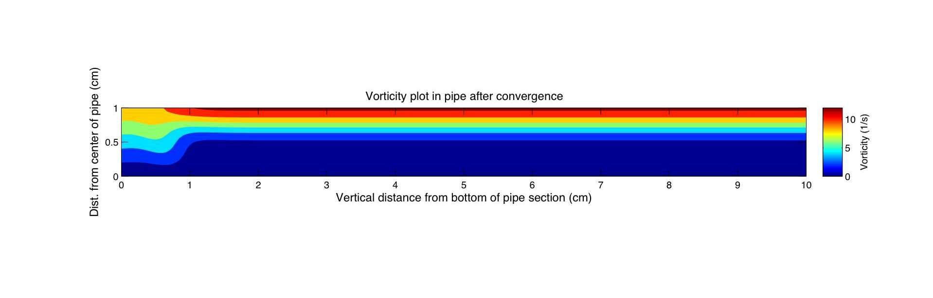
This program solves the laminar 2D Navier-Stokes equations on a pipe using finite differences. This is done using cylindrical coordinates. It uses the equations in their vorticity-velocity form to avoid the issue of pressure checker-boarding or odd-even decoupling where the pressure field gets decoupled from the velocity field. This is normally resolved using a staggered grid. More information can be found in a great book by Patankar called: Numerical Heat Transfer and Fluid Flow. In each iteration, a new vorticity is explicitly calculated from the previous vorticity. Then the radial velocity is implicitly calculated from the Poisson radial velocity equation using the Bi-CGSTAB algorithm. Then the axial velocity and the new vorticity is calculated from continuity. The boundary conditions are: a parabolic axial velocity profile in the West wall, zero axial and radial velocity in the North wall, a symmetric boundary condition in the South wall and no changes in radial or axial velocity in the East wall. The solver stops or converges when the maximum fractional vorticity difference between two iterations is 1e-3. As can be seen from the vorticity plot after convergence, the vorticity is close to changing linearly as a function of the pipe radius as it does in the analytical solution to the problem.

The equations used are as follows:

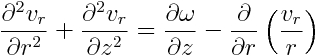
Vorticity transport:

Poisson radial velocity:

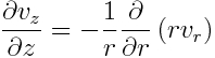
Continuity:

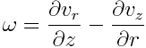
Vorticity:

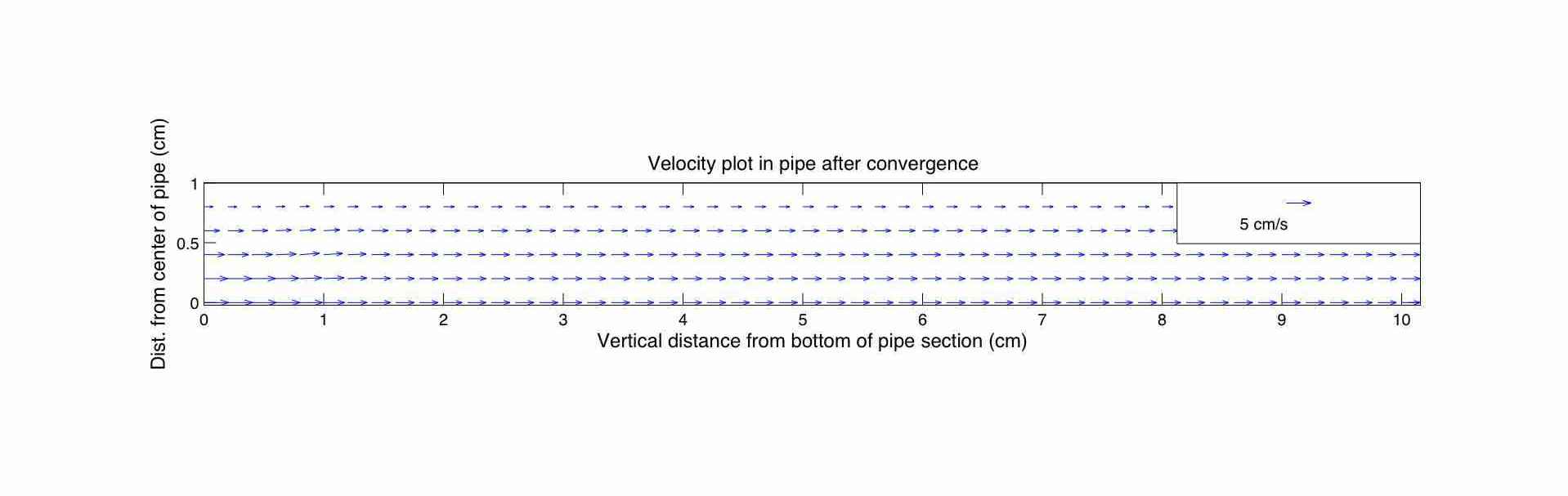
The code used to graph the velocity plot is a slightly modified code from the MathWorks' file exchange site: quivers.m. Here is the MATLAB program: vorticityNS.m.

The graph below shows the velocity plot after 200 iterations:

The graph below shows the vorticity plot after 200 iterations:

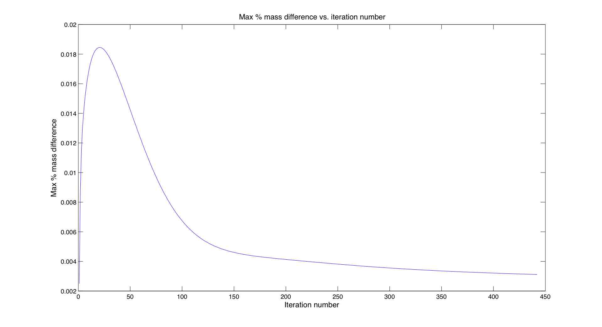
The graph below shows the maximum % mass flow difference with respect to the inlet:

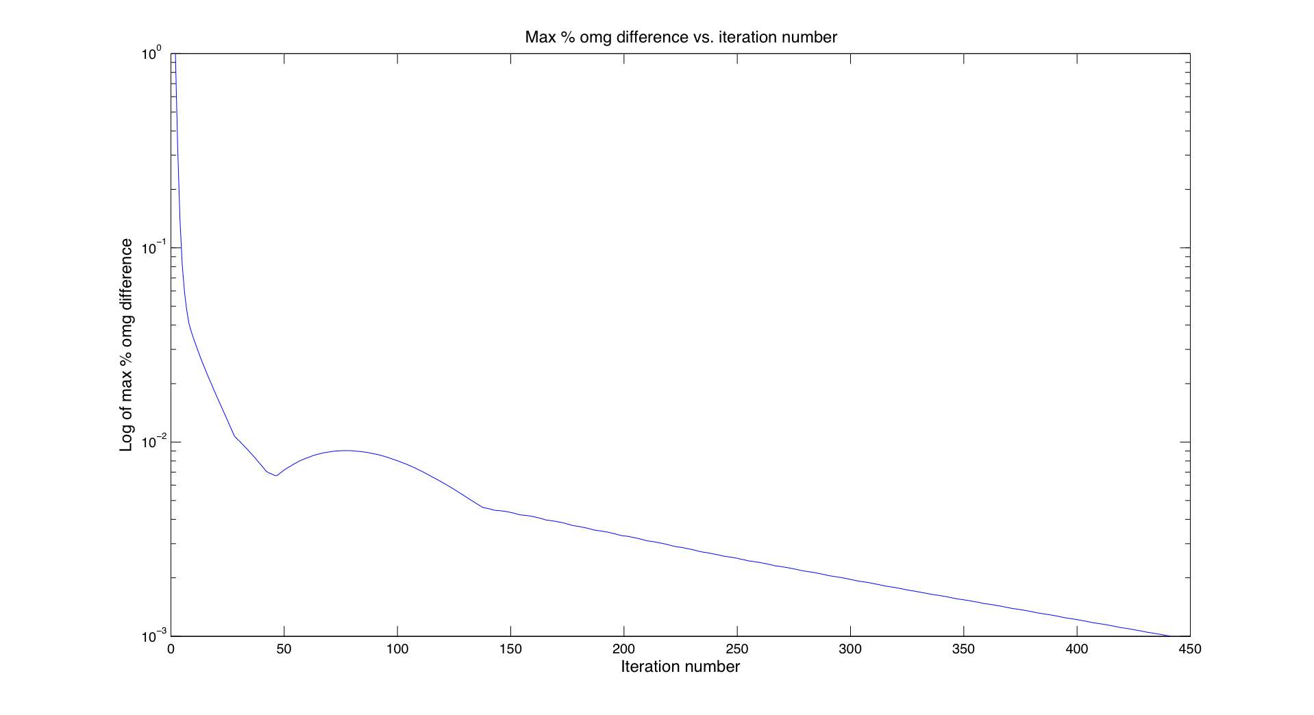
The graph below shows the maximum % vorticity change between subsequent iterations: